preliminary results from TOFr5 in Run-5
 
preliminary results from TOFr5 in Run-5
February 5, 2005 (first)
February 8, 2005 (update 1)
February 13, 2005 (update 2)
February 20, 2005 (update 3)
June 14, 2005 (update 4)
 
w.j. llope

Contents

1  First Look
    1.1  Introduction
    1.2  Analysis Details
    1.3  Results
    1.4  Summary and next steps
2  Update One
3  Update Two
    3.1  Start-side ToT
    3.2  Start-side Slewing
    3.3  Start-side Resolution
4  Update Three
5  Update Four
    5.1  New match trees
    5.2  Start-side correction from the match trees
    5.3  TOFp-style Stop-side correction
        5.3.1  Set-up
        5.3.2  Pion Selection
        5.3.3  ToT/Zhit fits
    5.4  Resolution results
Index

1  First Look

1.1  Introduction

RHIC Run-5 marks the first attempt at a number of important steps towards the full system. Most importantly, the NIM/CAMAC-based local trigger and DAQ systems provided by the TOFp system are replaced by new electronics (TAMP/TDIG/TCPU) that do the digitization on-board with respect to a 40 MHz clock. The data path to STAR DAQ over optical fiber also includes new electronics developed for the LHC. These are the first attempts at using these electronics in a running experiment.
At present TOFr5 HV and pVPD HV are controlled by the shift crew, and when TOF is included in runs the data collected by DAQ is saved on the so-called tof1 processor. These data are moved over to tofcontrol.starp by hand, where a "special.C" event reader collects all the TOF information from the daq file and writes all of the TOF data words to a text file.
The situation is quite chaotic at the moment. The major effort is on the development and refinement of the firmware installed on the TDIG and TPCU boards. The data format has changed several times in the week. The study of the very early data (Days 31-34) indicates several different data corruption problems at the < 1% level per event or less. Jo et al. are studying these problems carefully. What I did was simply discard any event that was corrupted, and concentrated on the rest. The goal was to see if the remaining data made any sense.

1.2  Analysis Details

A local version1 of special.C was used to extract the TOF data from the daq files. This code is the same as that kept up to date by Jo2 except that some additional text output was removed. The only words in the files written by my version is the (one line) event header, then two columns of data words (decimal DDLR number and 32bit data word as hex).
I then read these data using a simple CINT macro which produces a TTree of all of the event data after its been unpacked. This TTree is then used for all subsequent analyses.
The document needed to correctly unpack the data is Ref. [2]. The top 4 bits of each data word is the Packet Identifier. Using this identifier, the different types of data words can be unpacked into the more useful info such as channel number and data. The table at the end of this document spells out how to map a given TDIG number, HPTDC chip number, and HPTDC channel number to a detector channel index that goes from 0 to 191. We use the abbreviations LE and TE below to refer to Leading-edge data (in very-high-resn mode) and Trailing-edge data (in high-resn mode), respectively.
The DDLR values specify the data source: DDLR=1 means the TOFr5 tray, DDLR=2 means pVPD West, and DDLR=3 means pVPD East. For day 34 data and later, all three fibers are live and producing data. pVPD West is missing from data previous to this day due to a problem on that TCPU board.
"Geographical" words are included in the data stream beginning day 34. These are used to toggle a flag indicating which half of the tray the data is coming from. For data before day 34, one can easily use the "Separator" words to set this flag. The TDIG boards are read out in the following order: 1, 0, 3, 2, 5, 4, 7, 6 - where TDIG 0 is closest to the eta=0 end of the tray, and TDIG 7 is at the opposite end of the tray. TDIG boards 2 and 3 are masked out (no data will come from these) due to a problem. Its not likely this can be fixed during the run as the problem is inside the pole-tip.
The INL tables were obtained from Ref. [3]. The mapping from TDIG board name to TDIG position numbers in the tray is given in Ref. [4]. Each INL file contains either 1024 values (for very-high-resn TDCs) or 256 values (for high-resn TDCs). The lowest 10(8) bits in a LE(TE) data word are the INL bin number, which is the first column in an INL file. The Float in the second column applies to the data word itself to remove the INL. While i am reading in and applying the INL correction, none of the results discussed below use it. Post-INL correction, the TDC bin widths are 24.4(97.6) ps per bin. The dynamic range is 21(19) bits in very-high-resn(high-resn) mode, or ~ 51 microsec in both cases.
The results below were obtained from 502,705 events collected in Runs 06034014, 06034015, 06034016, 06034017, and 06034108. As mentioned above, events with any of the several types of data corruption errors were not processed.

1.3  Results

The number of bytes read out in each STAR event is shown in figure 1. The mean value is 872 bytes.
./plots/nbytes.jpg
Figure 1: The number of bytes of TOF data per event.
The distribution of packet identifiers is shown in figure 2. Packet identifier values of 4 are LE words, 5 are TE words, 12 are geographic words, 14 are TDIG separators, while 10, 11, and 13 are trigger headers or tags. There are thus, on average, sixteen LE TDC words per event (from all 3 DDLRs). The majority of these hits come from DDLRs 2 and 3 (the two sides of the pVPD). Interestingly, the number of TE TDC words is similar but not exactly the same - it's apparently ~ 5% smaller than the number of LE hits (more on this below).
./plots/PacketIdentifier.jpg
Figure 2: The distribution of packet identifier values.
The number of LE data words per event from the TOFr5 tray is shown in figure 3. The mean (including the zero bin) is ~ 3 LE stops per STAR event. Approximately 200k events ( ~ 40% of the total) have no stop-side hits.
./plots/hndataLEddlr1.jpg
Figure 3: The number of LE data words per event from the TOFr5 tray.
The number of LE data words per event from the start detectors is shown in figure 4. The left(right) frame depicts the distribution for the west(east) pVPD. The mean number of data words including the zero bin is in the range 6-7. Thus the ~ 16 LE data words per event comes from the various DDLRs in relative amounts tray:west:east of approximately 3:6.5:6.5, on average (in the mostly STAR-minbias Cu+Cu events analyzed here). There's a very weak (insignificant) tail to the distribution for the east side, but not on the west.
While there are 6 detector channels total in the pVPD, the STAR trigger for the present data set is primarily minimum bias. So this (large) mean value of 6-7 pVPD LE words per STAR event is more indicative of the large probability for multiple LE words per detector channel per event. Note the "timing windows" presently set up in the firmware are, quote, wide. For these data one thus needs an algorithm for selecting the correct hit to use from possibly several read-out in the event for the same detector channel (more on this below).
./plots/hndataLEddlr2.jpg  ./plots/hndataLEddlr3.jpg
Figure 4: The number of LE data words per event from the start detectors. On the left is the West (DDLR=2) and on the right is the East (DDLR=3).
Applying the maps at the end of the fiber data format allows one to produce hit patterns versus the Tray detector channel (0-191), where channel 0 is the first pad on the first MRPC from the eta=0 end, and 191 is the sixth pad on the 32nd MRPC closest to the eta ~ 1 end.
This hit pattern is shown in figure 5. In the top(bottom) frame is the number of LE(TE) data words versus the tray detector channel as the black histograms. The periodic pattern of groups of 6 in this histogram is expected due to "cross-talk" inside the MRPCs. Seeing this pattern is a very strong indication that the maps in the fiber data format document are being correctly applied. The gap from 48 to 95 is the two TDIG boards that were masked out of the data stream. There are 5 channels that are dead in both the LE and TE data (36, 108, 139, 156, and 180).
The number of LE(TE) data words for which there was no accompanying TE(LE) word in the same event for the same detector channel are shown in the red histograms in the upper(lower) frames. This indicates that, in general, the matching of LE and TE words in the same detector channels in the same events is quite good. In the upper frame, there are approximately 9k LE words per tray detector channel, and of these only some tens of these words were not accompanied by a TE word in the same detector channel ( << 1%).
The situation is less clean in the other direction. In the lower frame, one sees that a given TE hit is unaccompanied by a LE hit in the same channel at the 1% level. It therefore seems more appropriate to loop over LE hits and associate the TE data to the detector channels with LE data, rather than the other way around.
./plots/tread1.jpg
Figure 5: The LE and TE hit patterns versus the tray detector channel.
Now that it was clear that all the maps were being correctly applied, and that the LE and TE data match up well to each other in specific detector channels, it was time to start looking at the time stamps themselves. The first plot of this kind made is shown in figure 6. Here I selected events in which there was exactly one valid time stamp for pVPD East detector channel 0 (12 o'clock) and exactly one valid time stamp for pVPD East detector channel 1 (4 o'clock). The figure depicts the correlation of these two time stamps over the entire dynamic range of the LE data (each axis spans 50 microsec). The extremely strong band on the diagonal is a very strong indication that many of these time stamps are indeed useful physics data.
./plots/pvpd01corr.jpg
Figure 6: The correlation of the time stamps in two different pVPD detector channels in events in which there was one valid LE stop word for each detector channel.
The difference between these two LE time stamps in the same event is shown in figure 7. Similar plots can be produced for any pair of pVPD detectors on the same side of STAR - all pVPD detector channels appear to be producing valid and highly-correlated LE times. There are clearly offsets, as expected, as seen from the displacement of the peak from zero. While this distribution is not Gaussian (no corrections were done for this plot), the central core of these peaks have standard deviations for any pair of pVPD channels on the same side of STAR that are typically in the range of 20-30 very-high-resn bins, or approximately 500-700ps. This is excellent considering that this is roughly the resolution one expects if the INL and the PMT slewing corrections have not yet been applied.3
./plots/pvpd01corrd.jpg
Figure 7: The difference between the LE time stamp in pVPD (east) channel 0 and that from pVPD (east) channel 1, in events for which there was exactly one time stamp in each of these two detectors channel (without any other cuts).
Now that the detector mapping, LE to TE data matching, and start-side time stamps all appeared to be reasonable, I moved onto checking the correlations between the start times from the pVPD to the stop times from the TOFr5 tray (i.e. time correlations across DDLRs). A high degree of correlation would indicate that important and tricky aspects of the electronics related to the local clocks and resets was working.
To make this correlation, I first needed the event start time. This requires some selection of the hits to use for a given start detector channel, as there can be many per event. After staring at the start data for a while, it became clear that, to a reasonably good approximation, the first hit in given pVPD detector channel is generally the correct one. This particular "outlier rejection" algorithm is the simplest one possible, and can certainly be improved (I have a few ideas on what to try here).
Once the "acceptable" start-side hits in a given event have been identified, the East and West time averages are calculated separately (for those events where there was at least one detector channel with a valid LE data word). Following this, if there was at least one lit pVPD detector channel on each side of STAR in this event, the start time was set to the average of the east and west average times.
The distribution of event start times is shown in figure 8. The abscissa spans the entire 50 microsec dynamic range of the LE TDCs. TPC track information, specifically the primary vertex location obtained from the tracking, will be required to make sense of the shape of this distribution. Some fraction of the tail-off near the two extremes can certainly be the result of the fact that my present algorithms do not "wrap around" in TDC data space (i.e. to find/keep hits that are in fact near-time but for which the TDC bin counter has reset in the interim). The bump at start values near values of 1M is not yet understood. The event-by-event values of Zvtx from the tracking is needed to make more progress in understanding these trends.
./plots/tstart.jpg
Figure 8: The start time distribution.
The correlation of the event stop times from the TOFr5 tray to the start time so calculated from the pVPD is shown in figure 9. Again, an extremely strong correlation along the diagonal is seen. The both axes span the entire 50 microsec dynamic range of the LE TDCs, hence the entire TOF physics program lives inside a very small region of each bin on the diagonal in this plot (each bin here is 400 ns wide).
./plots/toflemstart.jpg
Figure 9: The correlation of TOF stop-side time stamps to the start time calculated from the pVPD time stamps in the same events.
The difference stop time minus start time in units of very-high-resn TDC bins is shown in Figure 10. All stop-side detector channels are included in this plot, as are all types of pVPD starts (i.e. specific number of lit pmts on the east and west in the event). One sees a very prominent grouping of the stop side time stamps after a specific time interval has elapsed relative to the event start time in the same event.
./plots/toflemstartd.jpg
Figure 10: The time difference TOFr5 stop time stamps minus the event start time calculated from the pVPD time stamps in the same events.
The structure in this plot is due to stop side offsets, which are not yet treated in the analysis (they are automatically treated in the stop-side calibrations once the track information is available). This is apparent from figure 11, where the stop minus start time differences are plotted versus the TOFr5 detector channel.
./plots/toflemstartd_itc.jpg
Figure 11: The time difference TOFr5 stop time stamps minus the event start time calculated from the pVPD time stamps in the same events, versus the TOFr5 detector channel.
Note that while there is no tracking information available at the moment to explore the timing resolution on the stop side, one thing suggested by figure 11 involves the performance of the various MRPC-retermination approaches attemped in the TOFr5 FEE. Each TAMP/TDIG combination (8 total, 24 detector channels each) uses a different approach. This figure seems to suggest that the MRPC termination schemes used in TAMP/TDIG positions 4 and 6 are working very well, while those at TDIG positions 0 and 1 are not working well at all. One can practically see LE ringing at those locations by the separate horizontal bands. This is not to imply that this can't be cleaned up at some level in subsequent calibrations.
Based on figure 10, I set a window that starts 3000 very-high-resn bins ( ~ 73 ns) after the event start time, and closes another 3000 bins later ( ~ 146 ns after this start time). Relative to figure 9, this implies a slice along the diagonal (and offset vertically from it by 73ns) that is only ~ 1/10th of one percent as wide as the (50 microsec) full range of the axes in this figure. The probability that a LE stop time stamp falls into this very narrow time slice relative to the event start time is shown versus the TOFr5 detector channel number in figure 12.
./plots/tofnstampscorrrat.jpg
Figure 12: The fraction of the total number of stop-side LE data words that are contained within a 73ns-wide window that begins(ends), event-by-event, 73ns(146ns) after the event start time (calculated using the start-side time stamps).
Despite the very-wide trigger matching windows, the majority of the LE stop times are very tightly correlated with the start time defined by the pVPD time stamps in the same event. These data are thus apparently quite pure (up to a factor of ~ 2, while the "incorrect" hits appear to be easy to recognize and reject).

1.4  Summary and next steps

These results seem to imply that the majority of the TOF Run-5 data words collected with the completely new clock-based TAMP/TDIG/TCPU approach on TOFr5 and both pVPD start detectors, and then read out using an also completely new optical fiber electronics path and protocol, seems to produce absolutely valid and sensible data for TOF Particle Identification.
Most of the data words seem to be highly correlated with each other, even across fibers (start detectors versus MRPC stop detectors). It seems then that we want to get into the normal data-stream as soon as possible. At least so far, this looks like decent (real) data.
A little less than one-half of the stop side hits saved to the datastream are "late," and generally uninteresting, due presumably to the wide trigger-matching windows presently in use in the firmware. These outlier time stamps are however relatively easy to recognize and reject. There does not appear to be an urgent need for defining tight(er) trigger-matching windows in the firmware. Our average data volume size with all three fibers active and wide matching windows is < 1 kB.
The near-term goals are:

2  Update One

The first two goals outlined in section 1.4 are now implemented. These were to implement the INL correction and a start-side outlier rejection.
The INL correction is read in and applied to all data words (all DDLRs). The HPTDC mapping was checked by filling two plots per HPTDC - one is the INL table read from the files of Ref. [3], and the other is the INL correction as it is applied as part of the event loop. In the former, the map INLfile to HPTDCnumber is hardwired based on Ref. [4]. In the latter, the INL bin number and HPTDC number is unpacked from the data word, and the HPTDC number is mapped onto the INL file number. The INL correction for this data word is then the INL value (from the file) for the given INL bin number.
To check that the INL values are being correctly applied to the data, the two INL curves (that read-in and that applied) are plotted versus the INL bin number (in a TH1F and a TProfile, respectively). A typical plot of this kind (there are 40 of these total), is shown in Figure 13. The INL corrections for a LE TDC (HPTDC=0) are on the left, and a TE TDC (HPTDC=3) on the right, versus the INL bin number. The black histogram is the table as read from the files, and the red points are the table as applied to the data during the event processing.
./plots/INLcompareLE.jpg  ./plots/INLcompareTE.jpg
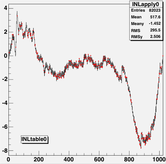
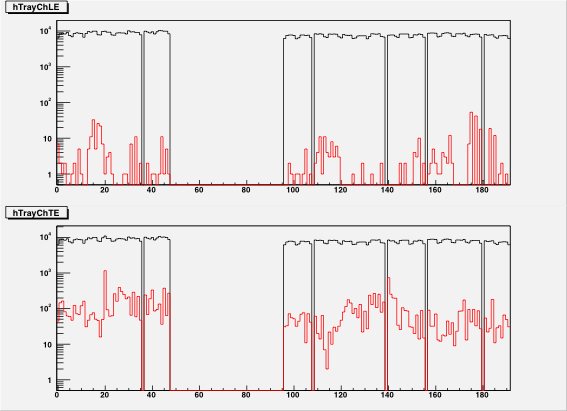
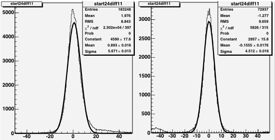
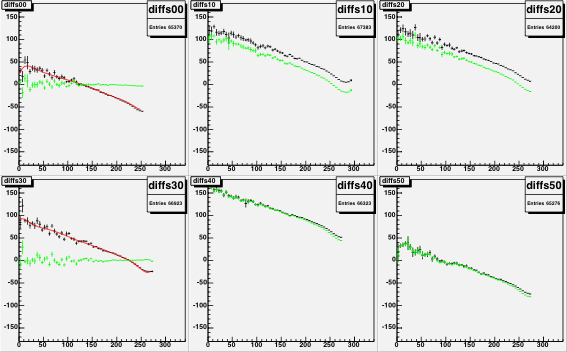
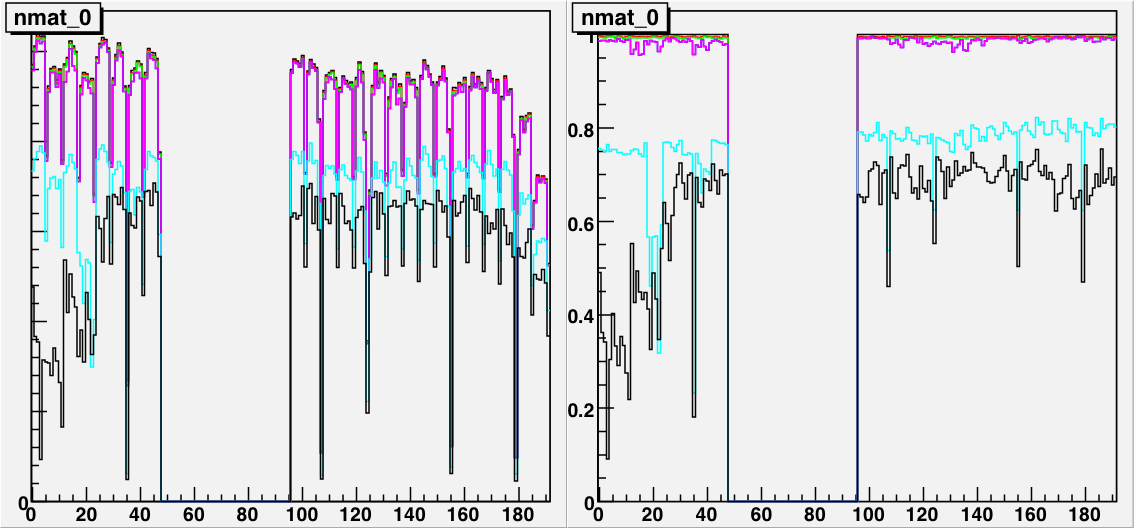
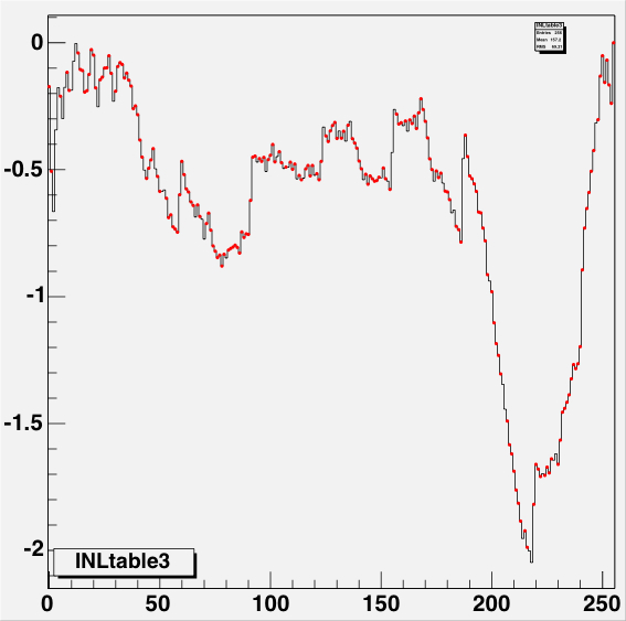
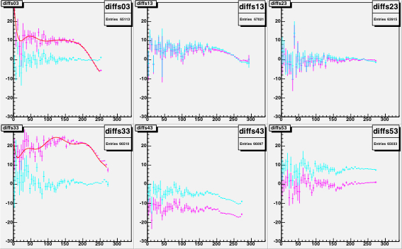
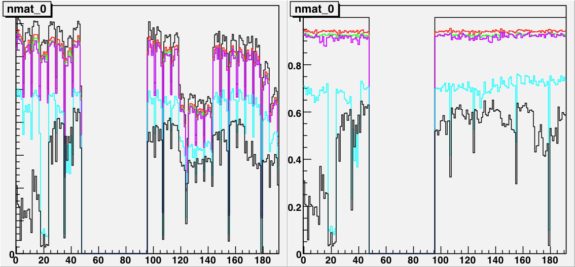
Figure 13: The INL corrections for a LE TDC (HPTDC=0) on the left, and for a TE TDC (HPTDC=3) on the right, versus the INL bin number. The black histogram is the table as read from the files, and the red points are the table as applied to the data during the event processing.
Similar comparisons are obtained from the other 39 TDCs in the system. With the INL under control, the next goal was the implementation of a start-side outlier rejection algorithm.
This is performed as follows. As before the earliest (LE or TE) time stamp for each pVPD detector channel is identified. All subsequent time stamps in the same detector channel and in the same event are discarded.
In section 1.3, all pVPD detector channels that were assigned a data word on this basis were allowed to participate in the calculation of the event start time. The result is Figure 8, which has some disturbing trends. The distribution is not flat (as it should be), and there a few peaks in the distribution (e.g. near channel ~ 1M) which should not exist.
The present algorithm goes a step further. If there was only one lit PMT on a side after the initial selection of hits, that PMT and time stamp is accepted as valid and used in the calculation of the start time. If there were 2 or 3 lit PMTs on a side after the initial selection, then all pairwise time differences between any two of the two or three lit PMTs is calculated. Any pair with a absolute difference less than 200 Very-high-resn TDC bins is assumed to be a pair of two time stamps, neither of which are outliers.
The start time distribution following the outlier rejection is shown in Figure 14. It is now flat, as expected.
./plots/tstart_outliercuts.jpg
Figure 14: The start time distribution following the start-side outlier rejection algorithm.
Also improved significantly is the matching from start-side to stop-side. The probability that a LE stop time stamp falls into a 73ns-wide time slice relative to the event start time (calculated without outlier rejection) is shown versus the TOFr5 detector channel number in figure 12. The efficiency seen is approximately 55%.
The same plot but now including outlier rejection in the calculation of the start time is shown in figure 15. With the improved measurement of the event start time resulting from the outlier rejection, this efficiency increases significantly to near ~ 65-70%.
./plots/tofnstampscorrrat_OC.jpg
Figure 15: The fraction of the total number of stop-side LE data words that are contained within a 73ns-wide window that begins(ends), event-by-event, 73ns(146ns) after the event start time (calculated using the start-side time stamps including outlier rejection).

3  Update Two

The last two goals mentioned in section 1.4 are now implemented. These were to study the Time-Over-Threshold values, and look into the possibility that these might support a slewing-correction. The ToT distributions on the stop-side are of special interest, given the various approaches used on TOFr5 to address the MRPC/TAMP termination issues. Slew-correcting the TOFr5 stops data will be a chore, as every group of 4 MRPCs (1 TAMP/TDIG) looks different (see figure 11). I put off until later studies of the stop-side ToT values and in the following concentrate on the start-side data. On this side, the kinematics of the particles of interest are such that direct measurements of the timing resolution of the system can be performed with the start-side data alone (no tracking or other information is needed). This is an often underappreciated benefit of having a good start system that also uses the same electronics as is used on the stop side. A realistic estimate of the timing resolution from the start-side in the Run-5 data taken by the new clock- and HPTDC-based digitization electronics would go a long way to show the basic health of the system, since the same electronics and read-out is used on the stop side.
In the present Cu+Cu data, the pVPD is getting lit up, as it did in the previous Au+Au runs. In these previous runs the pVPD detectors regularly achieved a sub-50ps resolution on the event start time (down to 24ps in central Au+Au collisions). Thus, from the standpoint of the detectors themselves, the signals in the present Cu+Cu collisions are large and hence the detectors' contributions to the (start-)timing resolution is relatively small. These detectors are exactly the same as in the previous runs, the only thing that has changed is the front-end, digitization, and read-out electronics.
We expect a good start-timing resolution post-corrections in Cu+Cu. Thus, we need not wait until calibrated STAR data (tracks etc.) are available (and perform a full start- and stop-side PID analysis) to gain insight into the basic functionality of all the new digitization and read-out electronics on TOFr5. If the start resolution extracted at this early stage from the pVPD data itself is poor, this system as a whole probably won't work well for PID, no matter how carefully we try to optimize the subsequent track matching and stop-timing calibrations. Subsection 3.1 describes the start-side ToT data, subsection 3.2 discusses the first attempt at a start-side slewing correction, and subsection 3.3 presents the start-timing resolution following this slewing correction.

3.1  Start-side ToT

The variable assumed to be related to the pulse height for the slewing correction in Run-5 is the Time-over-Threshold. This is ToT = 4*te - le, where te and le are the trailing- and leading- edge time values for a specific detector channel, respectively. The factor of 4 puts the trailing-edge data on the same time scale as the leading edge data - 0.0244ns per INL-corrected time bin.4
Given the HV gain set in use on the pVPD and the fact that this is Cu+Cu, we expect the typical pVPD pulse heights are well above threshold. The ToT distribution one would expect would thus have a peak at some value near some tens of nanoseconds. Shown in figure 16 are the ToT distributions for the six pVPD start detectors - East(West) 1 through 3 are left to right across the top(bottom).
These show several of the expected trends. The trailing edge times do trail the leading edge times in the same detector channel (ToT values are > 0), as expected. Also, as expected based on the fact that the typical pulse heights are well above threshold, there are relatively few counts for "small" pulse widths, and the probability for specific pulse widths increases for increasing pulse widths, forming maxima for widths of 20-30ns.
./plots/startToT.jpg
Figure 16: The ToT distributions for the six pVPD start detectors, East 1 is on the upper left and West 3 is on the lower right.
However, the shape of the distributions near these maxima is disturbing. One expects a distibution that tails off on both sides of some intermediate peak, but instead the distributions appear to cut-off for pulse widths larger than a maximum value of ~ 25-27 ns. Each pVPD channel shows a certain number of sharp peaks immediately above these widths which were also not expected. These peak features (which occur in different numbers and at different time values in the different pVPD detector channels), and the apparent cut-off near ~ 25-27 ns indicate a problem. We appear to be losing the ToT information for the largest pulses, which is unfortunate since it is these that lead to the best timing performance. These detector channels cannot be slew-corrected when the event's ToT values are in this strange upper region.
This ToT cut-off effect was then discussed within the group and is now interpreted as being caused by the input protection circuit on TPMT (the start-side's equivalent to TAMP on the stop side). Pulses that are larger than ~ 4V fire this circuit, which cuts off the top of the pulse at this voltage but still passes the lower section of the pulse to the discrimination/digitization circuitry. However, when this circuit fires, it drops to zero impedance, which inverts & reflects the signal as it comes in. The reflected/inverted pulse then travels back up the signal pigtail cable ( ~ 8.5 ft, ~ 13ns long), sees the large resistance of the PMT base, and reflects again (but does not invert). After another ~ 13ns this inverted signal returns back to the front-end electronics, where it destructively interferes with (what is left of) the original signal. This drops the apparent pulse below threshold at this point, and hence cuts off the ToT values there. Twice the signal pigtail length is ~ 26ns, this is (up to small channel-dependent offsets) precisely the value of the ToT cut-off that is observed.
In the access expected this wednesday (if not before) we will install 50 Ohm feed-through terminators at the pVPD PMTs. This will kill the reflected pulse when it returns to the PMT in those events where an input protection circuit fires. We hope to see that the result of this will be the removal of the effective cut-off in figure 16, and hence a more efficient and higher-quality slewing corrections.
We reduced the pVPD gains during last wednesday's access, in order to both reduce the chance the input protection circuit fires and also to effectively increase the probability a given event's ToT is in the useful range bealow ~ 25ns. As TOFr5 joined the full STAR data-stream also on that day, the TOF data collected since then must now be obtained from more traditional but slower sources (HPSS or the online event pool). I pulled down ~ 220k events from day 42 and processed them on the rcas machines using the same evp reader and subsequent analysis codes. The results obtained from the day 42 data (at lower gains) will be discussed alongside the results from the day 34 data (used throughout the rest of this document) in the following sections.
Until this reflections problem is solved at the next access, I will concentrate in the following on the data where the start-side ToT values are "on-scale" (ToT[ < || ( ~ )]25 ns). The existence of a correlation between these ToT values and the leading-edge times in the same channels in the right direction (i.e. small pulses are later than large ones) would be a very good sign that the ToT values are meaningful. This is investigated in the next subsection.

3.2  Start-side Slewing

To avoid possible sources of bias, slew corrections of the start detectors typically study a time difference, or a difference of time averages, across different detector channels in the same event. The dependence of such a time difference on the slewing measure - previously the pulse area (ADC) now the pulse width (ToT) - is the direct measure of the pulse slewing effect and the best means to correct for it. When there are lots of hits (Au+Au or Cu+Cu), the most effective differences of time averages to use for a slew correction are the "1- < 2 > " difference, or the " < 2 > - < 4 > " difference.
The former requires all 3 detectors on one side to fire in the same event, the latter requires all six detectors fired. In both cases, the slewing correction functions obtained from these events can be applied to the same PMTs in all events. The so-called Event Class index is plotted over the 220k Day 42 events in figure 17, after a cut requiring there was at least one lit detector on each side of STAR in the event. This index indicates how times there was a specific pattern of lit PMTs in a sample of STAR events. Indices 0 to 8 are the nine possible combinations where there was exactly one lit PMT on each side- index 0 means the two that fired was East 1 and West 1, while index 8 means that the two that fired was East 3 and West 3. Index 48 means all six detectors fired in the event.
./plots/ind_EvClass.jpg
Figure 17: The frequency distribution of the event class index over 220k day 42 events, after the requirement that at least one start detector channel was lit on each side of STAR in the event. For the details, see the text.
The "1- < 2 > " time difference can be formed on each side of STAR separately. The time difference of interest is the time from one detector minus the average of the two times from the other two detectors on the same side in the same event. The latter forms the < 2 > average from one detector on each side of STAR (e.g. East 1 and West 1), while the < 4 > average is over the other 4 detectors (2 on each side) in the same event.
According to figure 17 all six start detectors are lit in the majority of the events. For the following, I only fill the histograms that will later be slew-fit in these 6-detector events. I could gain some statistics in the "1- < 2 > " method by including events where the side of interest was fully lit but the other side wasn't, but the sample sizes are already plenty large and these 6-detector events should be cleaner anyway. Again, the fit parameters obtained from fitting the event class 48 events also apply to the events in all other classes (up to offsets possibly, but which are eaten by the stop-side calibrations).
The "1- < 2 > " time differences for all six pVPD detectors are shown in figure 18 versus the ToT values from the day 42 data. There is a wide but unmistakable correlation in the scatterplots of these variables (not shown), and this correlation has the right trend (small signals are later). The profile histograms of these correlations are what is shown in this figure as the black points. One sees what looks like perfectly standard slewing curves.
./plots/start0_day42.jpg
Figure 18: The start-slewing distributions versus the ToT for the six pVPD PMTs. For the details, see the text.
A start-slewing correction was then attempted. This starts by fitting the two left-most frames in figure 18 (East 1 above and West 1 below) with polynomials versus the ToT value, and then using those polynomials in subsequent passes through the data to remove the dependence of this differences on the ToT values. The fitted functions resulting from this first pass are seen in this figure as the red curves. The second pass applies these two fit functions to East 1 and West 1, and then calculates updated values of the "1- < 2 > " time differences for all six detectors (on each side of STAR separately). These are shown in this same figure versus the ToT as the green profile histograms.
In this second pass, these updated time difference curves are then fit for East 2 and West 2 versus the others, where the East 1 and West 1 values are the updated ones after the first pass. This results in a second set of two fit functions which will be applied to East 2 and West 2 in subsequent passes. and an update to all six time difference curves. In the third pass, East 3 and West 3 are corrected for the first time, and the values in the "2" averages here have all already been corrected once.
./plots/start3_day42.jpg
Figure 19: The same as figure 18, except after the fourth calibrations pass. Note the vertical scale was reduced by a factor of ~ 6 for this plot compared to figure 18. For the details, see the text.
Three passes remove the majority of the start-side slewing. The range of time difference values drops from tens of very-high-resn TDC channels to a few. This is seen in figure 19, which shows the same slewing curves after the 4th pass through the data. Note the vertical scales were reduced by a factor of ~ 6 for this plot relative to figure 18.
Additional passes make additional improvements in smaller and smaller amounts in groups of 3. After 10-12 passes the resulting start resolution no longer improves, so one can terminate the calibration passes at that point. The function applied to the data for each detector channel is the sum of the fit functions from each pass. The start-timing resolution one thus obtains following for the day 34 and day 42 data (separately) is discussed in the next subsection.

3.3  Start-side Resolution

Based on the experience with these same pVPD detectors in the previous Au+Au runs (digitized using long cables and TOFp's very well-understood CAMAC DAQ system) I would expect a start resolution for the present minimum bias Cu+Cu collisions in the range ~ 50-80ps. The start time is the average of the east and west times, which for the event class 48 events that I'm concentrating on now is the average over all six pVPD detectors.
The " < 2 > - < 4 > " time difference distribution following the start-side slewing corrections (and the INL calibrations) is shown in figure 20 for the 520k day 34 events on the left and the 220k day 42 events on the right. The standard deviation of this quantity for day 34(42) is 5.7(4.5) very-high-resn TDC channels, or ~ 140(110) ps.
./plots/start24diff11_day3442.jpg
Figure 20: The " < 2 > - < 4 > " time difference distribution following the start-side slewing corrections for the day 34 data (left) and the day 42 data (right).
These distributions are not Gaussian, but note that we are accepting all STAR events here (all trigger types, and no e.g. Zvtx or other standard sanity cuts) and also averaging over all event centralities (these data are mostly minimum bias Cu+Cu). The full analyses of these data in the STAR reconstruction chain won't suffer from any of these shortcomings. One also notices in the figure that a few percent of the events calibrate into separate stable peaks (e.g. near -45 ( ~ 1ns) in the right frame of figure 20). I don't think this is a bug in the calibrations algorithm, as that code is quite simple and has been used in similar forms successfully for the data from the previous RHIC runs. It appears here in some channels on the 4th pass (the first one after that when all 3 dectectors on a side have been treated once), and the scatterplots are featureless in the previous passes. This is perhaps the first indication that the simple outlier rejection algorithm used in section 2 needs to be optimized further. For example, the window used (+/- 200 bins, or about +/- 5ns) was set wide in order to insure that simple offsets would not confuse the rejection algorithm. It will be interesting to see how much tighter this window could be made and still retain the same efficiency for finding the correct start time in the event.
It may not be obvious just yet, but figure 20 is extremely good news. This " < 2 > - < 4 > " time difference is related to the event start time (the average over all six calibrated times in the event) via a factor of sqrt(2/9), or 0.47. This factor, and the 24.4 ps/TDC bin calibration (post INL-correction) is applied and shown for the day 42 data in figure 21. The horizontal axis in this figure is in picoseconds.
./plots/startresn11_day42.jpg
Figure 21: The start time resolution inferred from the " < 2 > - < 4 > " time difference distribution following the start-side slewing corrections for the the day 42 data. The abscissa is in units of picoseconds.
According to this figure, the start timing resolution attained by the pVPD with the completely new DAQ and read-out systems in event class 48 events from day 42 is approximately 54ps. This is despite the fact that these are minimum bias events without good-event, trigger-type, or any other sanity cuts, and also despite the fact that the ToT cut-off problem forces me to concentrate on those (smaller) signals that have on-scale ToT values. As in figure 20, the distributions are not Gaussian, which is a very good sign, given all that we're accepting and averaging over right now.
The 54ps start time achieved for the present "dirty" sample of also minimum bias events implies that the new DAQ and read-out systems are working well. One would have to assume at this point that these same systems are also taking data on the stop-side that will support high-efficiency and high-resolution particle identification.
What is needed to proceed in this crucial next direction is simply an updated "event reader" for the offline code. This will allow us to immediately use Level-3 (fast-offline) tracks for early studies of the stop-side and the overall PID performance. Haidong and Jing are working on this reader now.

4  Update Three

In order to address the problem seen in figure 16, 50 Ohm feed-through terminators were added to the start-side signal path during the access on February 16th (day 47). In this section I investigate the effect of this change using  260k (min. bias Cu+Cu) events from day 48.
Shown in figure 22 are the ToT distributions for the six pVPD detector channels following the addition of the terminators. Comparing this figure to figure 16, one notices immediately the distribution has much fewer "features" than the previous version - the high-cutoff and the addition peaks above this cut-off appear to be gone. The position of the most-probable ToT values dropped by a factor of ~ 5, and are now near ~ 225 very-high-resn bins, or ~ 5.5 ns.
./plots/termToT_6048012.jpg
Figure 22: The ToT distributions for the six pVPD start detectors, East 1 is on the upper left and West 3 is on the lower right, following the addition of the terminators to the signal path.
As the distributions of figure 22 now seemed more physical, the same start correction procedure used in section 3 was then applied to the new data. The intermediate results from the (14-pass total) calibration procedure are shown in figures 23 and 24.
./plots/start0_6048012-16.jpg
Figure 23: The start-slewing distributions versus the ToT for the six pVPD PMTs after start-calibration pass 0, and following the addition of the terminators to the signal path. For the details, see the text.
./plots/start3_6048012-16.jpg
Figure 24: The same as figure 23, except after the fourth calibrations pass. Note the vertical scale was reduced by a factor of ~ 6 for this plot compared to figure 23.
Figure 23 shows the slewing data and fits after the first pass through the data. One notices in this figure that the slewing curves with the improved start-side ToT are now much more linear than they were previously (cf. figure 18). Figure 24 shows the results after the fourth pass through the data (out of 14 total). Note the vertical scales for figure 24 were reduced by a factor of ~ 6 relative to figure 23.
Following 12 passes through the data, the start resolution of the TOFr5 system following the addition of the terminators is shown in Figure 25. The timing resolution obtained - ~ 57 ps (min.bias Cu+Cu) - is still excellent and consistent with that seen in figure 21, while the efficiency of the start correction is increased ( ~ 10-20%) by the addition of the terminators.
./plots/startresn11_6048012-16.jpg
Figure 25: The start time resolution inferred from the " < 2 > - < 4 > " time difference distribution following the start-side slewing corrections for the the day 48 data (after the addition of the terminators). The abscissa is in units of picoseconds. See figure 21 for the same distribution post-calibrations from the day 42 data (before the addition of the terminators).

5  Update Four

Present versions of TOF matching codes under CVS are not functional for the Run-5 data. A "private" maker was developed by Jing and Haidong, and the result was a new style of match tree for both the 200 and 62 GeV data. While quite different from the trees used for Run-2 through -4 analyses, these trees contained the variables necessary to perform a stop-side calibration and make significant estimates of the total timing resolution of the TOFr5 system.
In this update, I start with these trees and then apply the TOFp-style calibration strategy (see TOFp NIM). These calibration codes were already existing and only rather trivial modifications were needed, such as those dealing the format of this private match tree, 41chs vs. 192chs, and so on.
In this update, there are a total of 633k(421k) matches available in the stop trees for the 200(62) GeV data, respectively.
General comments on the match trees are made in section 5.1. The start-side resolution as from the trees (using the same algorithm as described in section 3.2 above) is discussed in section 5.2. The TOFp-style stop correction approach was then applied in section 5.3 and the results are discussed in section 5.4.

5.1  New match trees

Brief history of these match trees:
As the original event.root files were no longer available at this point, new code was then needed to run the private match maker on the available micro DSTs. jing regenerated the same match trees with all of the geometry improvements. these trees are what is analyzed here.
These trees allows all star Zvtx-values, as well as other areas of "looseness" such as matches with ToT<0 or Abs(Zhit)>3.1cm. I presume the twist correction was incorrect in the production used to make these trees.

5.2  Start-side correction from the match trees

The start-timing correction discussed in section 3.2 above used local data that was collected early in the run when the HPTDC "trigger-matching" windows were very wide (25 microsec). The data for the present trees was only from that collected after the timing windows were reduced to ~ 1 microsec. Thus the detailed outlier rejection algorithms described above are less important for these data, and I presume only the "earliest" time stamps for each event were those passed to the match trees.
The distribution of so-called "Event Class" Indices is shown in Figure 26. This index is the same as that described in Ref [5]. and it indicates the specific pattern of pVPD PMTs that fired in an event. Event classes 0 through 8 are the nine possible combinations of lit PMTs in those events in which exactly one pVPD PMT fired on each side of STAR. Bin 48 gives the number of events for which all six pVPD PMTs fired in the event.
./plots/comp01.jpg
Figure 26: The event class index for the 200 GeV (blue) and the 62 GeV (magenta) Cu+Cu data from Run-5. Bin 48 gives the number of events in which all six pVPD PMTs fire in the event. Bins 0 through 8 are those for which exactly one pVPD PMT fired on each side (East and West) in the event.
In the 200 GeV data, > 90% of the events light up all six pVPD PMTs. The 62 GeV data has a much more significant population of events with < 3 pVPD PMTs firing on either side. The start timing resolution degrades significantly when going from right to left across this figure. The inclusive start-timing resolution for the 200 and 62 GeV data is shown in Figure 27. The resolution observed is approximately 51 ps and 83 ps, respectively, averaged over the full sample of minimum bias events available at each energy.
./plots/comp02.jpg
Figure 27: The start-timing resolution for the 200 GeV (blue) and the 62 GeV (magenta) Cu+Cu data from Run-5.
This value of ~ 50ps for the inclusive start resolution for the 200 GeV data is consistent with the estimates made using the Run-5 local data (see section 3.3 above). This was considered good at the time due to the unknown smearing to this quantity coming from the event centrality (these data are minimum-bias triggered by STAR).
This smearing can now be exposed using the values of nprimary from the start trees. The start-timing resolution in nanoseconds versus nprimary is shown the the 200 GeV data in figure 28. This plot shows that the timing resolution in the most central events is similar to that one gets by fitting just the core of the 1D plots (e.g. figure 27).
./plots/scomp01.jpg
Figure 28: The start-timing resolution in nanoseconds versus nprimary for indEvClass=48 events at 200 GeV.
I would have expected a somewhat better resolution for the most central collisions than is observed. This may be an indication of the TDIG timing cross-talk that has recently been seen on the bench.
This will be investigated in more detail over the next few days and the results summarized in a subsequent update.

5.3  TOFp-style Stop-side correction

The approach used here is the same as that used for the TOFp data from Run-2 [6]. This algorithm lives in 1/beta-space, becuase the high-quality tracking information from the TPC defines a powerful "standard candle" for the TOF stop-side slewing and signal propagation time corrections across the full momentum acceptance of the TOF system.

5.3.1  Set-up

The first thing we need is a crude timing offset in nanoseconds for each TOFr5 channel relative to the calibrated start time (also in ns) in the same event. We're just trying to get 1/beta "on-scale" here (which means somewhere close to 1). The total timing resolution is so bad at this point that getting the offset correct to 10% is perfectly sufficient.
The mean path length in cm for all matches versus the TOFr5 channel number for the 200 GeV (blue) and the 62 GeV (magenta) Cu+Cu data is shown in Figure 29. The low-(high-)eta end of the tray is on the left(right) side of the abscissa.
./plots/comp03.jpg
Figure 29: The mean path length for matches versus the channel number for the 200 GeV (blue) and the 62 GeV (magenta) Cu+Cu data from Run-5.
These average track-length values were tabulated for each MRPC module (32 total). In a subsequent pass through the data, these values of "Savg" were used to come up with a crude timing offset, "preoffset," via
       timeraw = letime - tstart;
       invbetaraw = vlight*timeraw/trklen;
       preoffset = (Savg/vlight)*(1.-invbetaraw);
where letime is the HPTDC time stamp for this match in ns, tstart is the calibrated start time (post start-ToT correction) in ns, vlight is 29.979 cm/ns, and trklen is the reconstructed total track length for this match obtained from the track reconstruction. The initial timing offsets extracted in this way are shown versus the TOFr5 channel number in Figure 30.
./plots/comp04.jpg
Figure 30: The initial timing offsets extracted using the values of Savg for each MRPC module (obtained from figure 29) for the 200 GeV (blue) and the 62 GeV (magenta) Cu+Cu data from Run-5.
These crude timing offsets are used to jump immediately into 1/beta-space via
       invbeta[0] = vlight*(timeraw + toffset[chanid])/trklen;
where toffset[chanid] is that shown in figure 30 and trklen is the total path length for this track. All subsequent stop-side corrections and PID assignments thus also live in 1/beta-space.

5.3.2  Pion Selection

The pion selection method used here to select the matches to be used to then extract the slewing and Zhit correction functions differs significantly from that used in the "BNL approach".
The mean TPC dE/dx (in keV/cm) for pions versus the momentum for the 200 GeV (blue) and the 62 GeV (magenta) data is shown in Figure 31. These mean values are used only as a (momentum-independent) consistency check on the pion selection done in 1/beta-space. The cut is loose (-0.6 keV/cm to +0.4 keV/cm relative to the pions), so the slight difference seen for the two beam energies is not so important.
./plots/comp05.jpg
Figure 31: The mean TPC dE/dx (in keV/cm) versus the momentum for the 200 GeV (blue) and the 62 GeV (magenta) Cu+Cu data from Run-5.
The action is really occurring in figure 32. In the upper left is the inverse velocity versus the momentum for all matches (with the only calibrations being the start correction and the definition of the crude channel-dependent offsets). The main peak is near 1 on the Y-axis since we chose offsets that insured this outcome. The upper right frame shows the matches defined as pions in the first calibrations pass through the data. In the two subsequent passes through the data (i.e. during the various slewing and Zhit calibration passes), the pion selection cut becomes tighter in 1/beta-space yet remains momentum-independent. The pion selection cut is set crudely in the first calibrations pass, is tightened twice in the next two calibration passes, and is then fixed for any subsequent passes.
./plots/pioninvbeta_200GeV.jpg
Figure 32: The values of 1/beta versus the momentum for the first 4 passes. In the upper left is that for all matches after only the application of the crude timing offsets. The upper right shows those matches accepted as calibration pions for the first calibrations pass (over ToT, see below). The lower left(right) shows those matches accepted as calibration pions in the second(third) calibrations passes (over Zhit and ToT again respectively.
The dE/dx mean values from figure 31 are used to set a pion consistency check above and beyond the 1/beta-space selection depicted in figure 32. The distribution of TPC dE/dx values versus the momentum are shown in figure 33 for the same conditions used in figure 32. These are, if you like, all matches, bronze pions (pass 0), silver pions (pass 1), and gold pions (passes 2 ans above) going from upper left to lower right.
./plots/piondedx_200GeV.jpg
Figure 33: The TPC dE/dx values for the calibration pion selection. The individual frames correspond to the same calibration passes as seen in figure 32.

5.3.3  ToT/Zhit fits

Matches flagged as calibration pions are used to fill specific TProfiles that will later be fit with a calibration function at the end of each pass. In the first calibrations pass, the quantity 1/beta-1/betaexpected(pi) is plotted versus ToT for each TOFr5 readout channel. At the end of this pass, this distribution is fit with a polynomial for each channel and the fit parameters tabulated for use in subsequent passes. Examples of the ToT fits in this first calibrations pass are shown in figure 34. One notices the quite different scales in ToT that exist in the different TDIG boards due to the different MRPC termination schemes employed under each TDIG.
./plots/AZfits_200GeV_0.jpg
Figure 34: Examples of the ToT fits performed after the first calibrations pass. The six frames correspond to one read-out channel from each of the six active TDIG boards on TOFr5 for the 200 GeV data.
In the second calibrations pass, the ToT correction functions from the previous pass are applied, and new TProfiles are filled in order to attack the Zhit dependence. Examples of these Zhit fits are shown in figure 35.
./plots/AZfits_200GeV_1.jpg
Figure 35: Examples of the Zhit fits performed after the second calibrations pass, where now the plotted pion 1/beta values are those after the initial ToT correction. The six frames correspond to the same read-out channels from each of the six active TDIG boards on TOFr5 as shown in figure 34.
The procedure continues in this way - ToT fit then Zhit fit then repeat - for 4 passes or so. A third pass is definitely necessary in this approach. Doing too many fit passes doesn't hurt. For the results below I stopped this ToT/Zhit fit iteration after 4 passes. Whether a third (or fourth) pass would help the BNL-style approach is an open question.

5.4  Resolution results

The stop-side calibrations are complete at this stage. While I work in 1/beta-space, one would like a resolution estimate in ns in order to touch base with historical expectations. The number 100 ps gets thrown around a lot. Anything in this ballpark results in a good efficiency to ~ 1.6 GeV/c for pi/K/p PID, and to ~ 2.8 GeV/c for (pi+K)/p PID.
To quote a timing resolution in ns, I thus convert the 1/beta-1/betaexpected(pi) distributions to a time scale via
       timelike = savgModule[kModule]*(1/beta-1/betaexpected(pi))/vlight;
and then fit these distributions with Gaussians. The total timing resolution versus the TOFr5 channel number thus extracted is shown for the 200 and 62 GeV data in figures 36 and 37, respectively.
./plots/resn_200GeV.jpg
Figure 36: The total timing resolution for the 200 GeV Cu+Cu data from Run-5 versus the TOFr5 channel number. The black points are for all calibration pions while the open points are for a specific set of golden track and golden match cuts (described below).
./plots/resn_62GeV.jpg
Figure 37: The same as 36, except for the 62 GeV data from Run-5.
The histograms of these timing resolution numbers over all active read-out channels are shown in the two following plots. The timing resolution histogram for all matches in the 200(62) GeV data is shown in the left(right) frames of in Figure 38. The total resolution observed is of order 108(151) ps over 144 channels at 200(62) GeV.
The timing resolution histogram for "golden" matches (described below) in the 200(62) GeV data is shown in the left(right) frames of in Figure 39. The total resolution observed for these matches is of order 100(137) ps over 144 channels at 200(62) GeV.
./plots/comp06.jpg
Figure 38: The histogram of calibrated timing resolutions across all active TOFr5 read-out channels for the 200 GeV (blue) and the 62 GeV (magenta) Cu+Cu data from Run-5.
./plots/comp07.jpg
Figure 39: The histogram of calibrated timing resolutions across all active TOFr5 read-out channels when including specific additional good track and good match cuts for the 200 GeV (blue) and the 62 GeV (magenta) Cu+Cu data from Run-5.
The cuts used to select "golden" matches are defined by the plots shown in figure 40. The standard deviation of 1/beta-1/betaexpected(pi) for matches with 0.5 < p < 1.5 GeV/c is plotted versus the track global dca (upper left), the number of primaries (upper right), Zvtx (lower left), and h (lower right). One sees tracks with dca > 1.5 cm, and events with |Zvtx| > 30 or so have a relatively poorer time resolution. Tracks with less than ~ 30 hit points also have a poorer time resolution. The cut used here to define golden matches was thus
       Zvtx > -10
       Zvtx < 30
       nfitpoints > = 30
       dca < 1.5

./plots/comp08.jpg
Figure 40: The standard deviation of 1/beta-1/betaexpected(pi) for matches with 0.5 < p < 1.5 GeV/c following all start and stop corrections versus the track's global dca (upper left), the number of primaries (upper right), Zvtx (lower left), and h (lower right).
The PID capabilities over all active read-out channels are indicated in the following two plots. In each plot, the TPC dE/dx is shown versus the momentum in the upper left for all tracks with 1/beta < 1.03. The upper right through lower right plots show 1/beta-1/betaexpected versus the momentum for pions, Kaons, and protons, respectively.
./plots/ipid_200GeV.jpg
Figure 41: The PID cuts for electrons (upper left) through protons (lower right) in 1/beta-space for the 200 GeV data.
./plots/ipid_62GeV.jpg
Figure 42: The PID cuts for electrons (upper left) through protons (lower right) in 1/beta-space for the 62 GeV data.
The calibration pion sample sizes for each TOFr5 read-out channel are shown for 200 and 62 GeV in figures 43 and 44, respectively. In each figure, the raw counts are shown in the left frame, and the right frame shows these normalized to the total number of raw matches. The calibrations functions obtained from the pion samples are of course applied to all good matches in a last pass through the data. The "PID" efficiencies are thus not shown in these figures - these just describe how matches are flowing through the selection criteria for calibration pions.
The Red, Green and Blue lines in these figures correspond to rejection of events or matches with
       ind_EvClass < 9
       TMath::Abs(vtx[2]) > 100.
       ToT < 0.
The magenta, cyan, and black lines shows the rejection by the first-, second-, and third- levels of pion selection (see figs. 32 and 33). Approximately 70% of the matches make it through all three levels of pion selection and are thus used for all of the stop-side calibrations.
The calibration sample size dives down at low-eta, and I'm in the process of investigating this. I also need to make the PID efficiency plots.
./plots/effi_200GeV.jpg
Figure 43: The histograms (left frame) and the calibration efficiencies (right frame) versus the TOFr5 channel number for the various stages of these calibrations for the 200 GeV data.
./plots/effi_62GeV.jpg
Figure 44: The histograms (left frame) and the calibration efficiencies (right frame) versus the TOFr5 channel number for the various stages of these calibrations for the 62 GeV data.

References

[1]
TOFr5 Design:
http://wjllope.rice.edu/ ~ TOF/TOFr5/Documents/tofr5.pdf
[2]
Fiber Data Format document:
http://www.rhip.utexas.edu/ ~ jschamba/TOF_Fiber_Data_Format.pdf
[3]
INL files location:
http://www.bonner.rice.edu/ ~ liuj/TDIG/calib-Oct-20-2004/inltable/
[4]
TDIG name information:
http://www.bonner.rice.edu/ ~ liuj/TDIG/tofrLVsetting/tofr-LV-list.doc
[5]
Description of ind_EvClass:
http://wjllope.rice.edu/ ~ WJLlope/-myPublications/CollabMtgTalk_20030811.pdf
[6]
TOFp NIM Paper:
Nucl. Inst. and Methods, Section A, 522, 252 (2004).

Footnotes:

1tofp@tofcontrol:/home/tofp/wjl/evp/special.C.
2tofp@tofcontrol:/home/tofp/tof/evp/special.C.
3In Run-5, we rely on Time-Over-Threshold information to do the slewing correction. The ToT is obtained by subtracting the LE time stamp from four times the TE time stamp.
4The use of ToT = te - le/4 and a time bin width of 0.0976ns would be completely equivalent.


File translated from TEX by TTH, version 3.38.
On 20 Jun 2005, 12:41.